cs代做_statistics代写-Mathematics and Statistics Computer Project

Mathematics and Statistics
Computer Project

statistics代写 Prove the following theorem: Theorem: The log optimal portfolio x∗ for a fixed distribution F satisfies the following necessary

Due on Sunday 10th November at 11:59pm on TurnitIn  statistics代写

• Submit exactly two files: a pdf with your report and m file with your Matlab code.
Report should be pleasant to read and include project formulations, descriptions and outputs (tables, plots, histograms etc), all answers and discussion should be there. Marking will be based on: accuracy, programming and presentation.

• Please do not write your name on any sheet.

• The deadline is a hard deadline in the sense that in case of a late submission (maximum up to 10 days), you will be deducted 5% of the total marks for each day of delay. This is non-negotiable, so make sure you submit in time; a submission on Monday the 11th at 12:01am will be an automatic deduction of 5%. It is your responsibility to check that your submission was successful.

MATH2070: Do all questions except Question 6.
MATH2970: Do all questions.

In this computer project you will be analysing real stock market data downloaded from Yahoo!Finance. The file Data_2013_2019.csv which you can download from Ed, contains the daily closing prices of the 30 stocks which make up the Dow Jones Industrial Average Index and closing prices of two indexes, Dow Jones Industrial Average Index and S&P 500 Index. Prices are recorded on a (business)-daily basis between 2/01/2013 and 30/09/2019.

There is one particularity with this time series: On 31st of Ausgust 2017 Dow and DuPont merged and were traded as a new entity DowDuPont, then in 2019 Dow spun off of DowDuPont and was added to the Dow Jones Industrial Average. Therefore only consider the 29 stocks without Dow (due to a short trading history).

All prices are in US dollars.  statistics代写

Correlations and the covariance matrix

1. Export the data into Matlab using csvread and/or readtable. This question investigates the correlations of the return rates of the 29 stocks. When analysing return rate data one has several choices. A commonly used variable is the logarithmic change of price or the so called log return rate: Let Skt be the price of k-th stock at time t, then consider Ykt = log Skt − log Sk(t−1) (wrt the natural base).

(i) Calculate the maximal correlation between the Yk, name and plot the two stock prices associated with the highest correlation as a function of time. On the graph present normalised time series so that they start from the same value 100 on 2/01/2013.

(ii) Calculate the minimal correlation between the Yk, name and plot the two stock prices associated with the smallest correlation as a function of time. On the graph present normalised time series so that they start from the same value 100 on 2/01/2013.

(iii) Visualise the correlation matrices for two subperiods: 1/12/2014–1/09/2016 and 1/09/2016– 1/02/2018 (you may use Matlab’s command imagesc). Can you spot differences? Plot the price of Dow Jones Industrial Average in the whole period. Can you relate it to your observations about the correlation matrices?

(iv) Plot the histogram of the correlation coefficients ρij for the two periods from the previous point. Comment on your result.

(v) Find the maximal risk (expressed via standard deviation) of the 29 stocks and the most risky stock corresponding to this value. Calculate the maximal correlation between the most risky stock and one of the remaining stocks, name and plot these two stock prices as a function of time. On the graph present normalised time series so that they start from the same value 100 on 2/01/2013. (Here work with the entire time series.)

(vi) Find the minimal risk (expressed via standard deviation) of the 29 stocks and the least risky stock corresponding to this value. Calculate the maximal correlation between the least risky stock and one of the remaining stocks, name and plot these two stock prices as a function of time. On the graph present normalised time series so that they start from the same value 100 on 2/01/2013. (Here work with the entire time series.)

Portfolio Theory  statistics代写

2. In this section we consider simple return rates, that is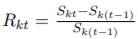Sk(t−1) , where Skt is the price of the k-th stock at time t. Carry out the following computational tasks for an unrestricted optimal portfolio P∗ consisting of the 29 stocks included in the Dow Jones for an agent who wants to invest $200,000 and has a risk aversion parameter t = 0.2.

(a) Compute the dollar investment in each of the stocks and the corresponding expected return and risk of P∗.
(b) Illustrate the problem graphically and plot on the same graph in the µσ-plane :

(i) The 29 stocks of the Dow Jones.

(ii) The minimum variance and efficient frontiers. Use a t-range |t| ≤ 0.35 for your display.

(iii) A plot of 1000 random feasible portfolios satisfying |xi| ≤ 20 (for each of the 29 stocks)and σi ≤ 0.05 for i = 1, . . . , 1000.You might notice that the random points occupy some region well-separated from the minimum variance frontier (MVF) - comment on this and explain why (This is a/the major part of the question).

(iv) The indifference curve of an investor with t = 0.2 and their optimal portfolio P∗.

3. Determine which investors shortsell in the market consisting of the 29 stocks, and which stocks they shortsell. Are there any stocks which no-one will shortsell or which everyone will shortsell?

4. Three funds with different risk profiles: In this question you will divide 29 stocks with respect to their risk profile into 3 funds. Sort stocks from highest to lowest risk (expressed via variance or standard deviation). Assuming that each stock has the same contribution to a given fund, form high-risk fund from the 9 most risky stocks, low-risk fund from the 10 least risky stocks and mid-risk fund from the rest.  statistics代写

(a) Compute expected returns and covariance matrix of the 3 funds.
(b) Let Pˆ be an unrestricted optimal portfolio consisting of the 3 funds for an agent who wants to invest $200,000 and has a risk aversion parameter t = 0.2.

(i) Compute the dollar investment in each of the stocks and the corresponding expected return and risk of Pˆ.

(ii) Plot on the second µσ-plane graph :

• The 3 funds.

• The minimum variance and efficient frontiers. Use a t-range |t| ≤ 0.35 for your display.

• The indifference curve of an investor with t = 0.2 and their optimal portfolio Pˆ.

• The minimum variance frontier and optimal portfolio P∗ from Question 2. Compare solutions P∗ and Pˆ to the two problems based on computations and graphs.
Capital Asset Pricing Model

5. Assume that the daily risk free rate in the studied period was 0.002906%. Suppose that Standard & Poor’s 500 Index is the market portfolio (S&P 500 Index prices are included in the data file). Make a new µσ-plane graph showing the risk free asset, market portfolio, and the Security Market Line. Compute the β’s of all relevant assets in this project (29 stocks, 3 funds, and two optimal portfolio P∗ and Pˆ from Questions 2 and 4). Plot these assets on the same graph. Identify assets with β’s greater than 1 and lower than 1. Comment on the result and describe what Portfolio Theory would recommend an investor to do.

Log Optimal Portfolio  statistics代写

In this section we consider logarithmic utility maximisation problem. As in Markowitz Portfolio Theory, there is a random vector of returns on n stocks R = [R1, R2, ..., Rn]. The objective is to maximise the expected logarithmic utility of the final wealth W1, i.e.,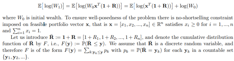

Note that the above expectation is computed with respect to the distribution of R¯ which is uniquely determined by F

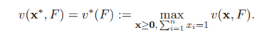
For a fixed F, a feasible portfolio x∗ that achieves the maximum of v(x, F) is called log optimal portfolio, i.e.,

6. (a) Show that

(i) v(x, F) is concave in x and linear in F,

(ii) v∗(F) is convex,

(iii) the set of log optimal portfolios with respect to a fixed F is convex.

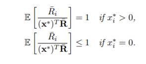
(b) Prove the following theorem: Theorem: The log optimal portfolio x∗ for a fixed distribution F satisfies the following necessary and sufficient conditions:

Hint: Using 6(a)(i) argue that log optimal portfolio can be characterised locally by an appropriate condition on the directional derivative of v in the direction from x∗
to any other feasible portfolio x.

更多代写： HomeWork cs作业     金融代考    postgreSQL代写         IT assignment代写     统计代写代写英国留学作业