
EE 430-Principles of Electromagnetic Fields H.O.
电子工程代考 the potential on all boundaries (i.e., at grid points corresponding to ix=1, ix=nx+1, iy=1:ny+1; and iy=1, iy=ny+1, ix=1:nx+1).
Instructions: 电子工程代考
- The project reports should be submitted to the homework collection slot (121 EE East) on Thursday 03/05/2020 before 4 PM (this is absolute deadline). Please include a cover sheet (this page) with you name and assignment questions, and a brief
description of your solution approach (including principal mathematical expressions) for each of the project assignments. Please include in your report copies of all codes you developed for this project. You are allowed to use your textbook, your own lecture notes, and MATLAB function sorEE430S20.m posted in EE 430 Project folder on CANVAS. Please review pages 93-110 of the textbook, and H.O.s #14 and #15 on solution of partial differential equations using finite differences before starting your work on this assignment. No other materials are permitted. You are allowed to discuss project assignments with your classmates only, but only on conceptual level. The completed project should be your own work. You are not allowed to share parts of the code or compare final results.
1. (20%) Find analytical solutions for the electric field E~ and potential V for an infinite cylinder of radius R uniformly charged with density ρ0. Assume that V =0 at the axis of the cylinder.
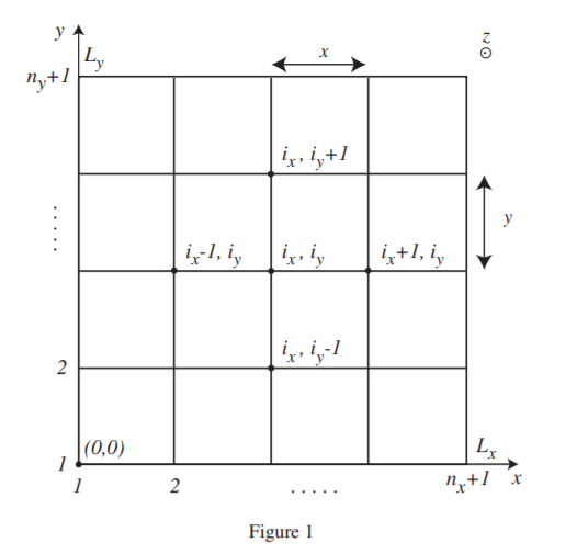
Assuming that z axis is parallel to the axis of the cylinder and that the cylinder is centered at the point with coordinates x0 = Lx/2 and y0 = Ly/2 in the center of the two-dimensional domain shown in Figure 1, find values of the potential and
electric field at grid locations. Define positions of grid points as x(ix)=∆x × (ix − 1) for ix varying from 1 to nx + 1, and y(iy)=∆y × (iy − 1) for iy varying from 1 to ny+1, where ∆x=Lx/nx and ∆y=Ly/ny. Plot scans of the potential and electric field
magnitude as a function of x at y0 = Ly/2 and as a function of y at x0 = Lx/2. You can use MATLAB functions contour.m, imagesc.m, quiver.m to plot two-dimensional distributions of the potential and electric field (vector and magnitude). Assume
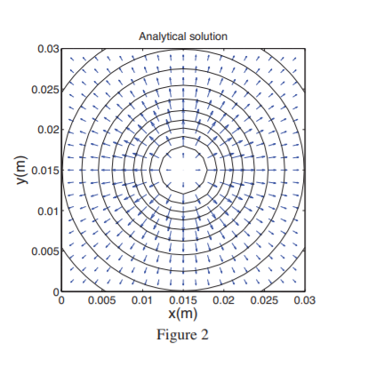
Lx=Ly=3 cm, R=Lx/6, ρ0=8.85×10⁻¹² C m−3 . It is useful to plot both potential (using contour.m) and electric field vector (using quiver.m) in the same figure, as illustrated in Figure 2, to visualize the relationship between the equipotential lines and electric field vector. Look at results for two resolutions nx=ny=20 and nx=ny=100.
2. (30%) Having reviewed H.O.s #14 and #15 verify that the two dimensional form of the Poisson equation 电子工程代考
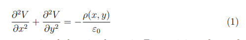
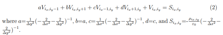
can be represented in the computational domain shown in Figure 1 in a form of five-point finite difference equation
Using successive overelaxation (SOR) method described on pages 179-181 of H.O. #15 find solution for the potential and electric field for the cylindrical charge distribution specified in the previous part of the project assuming constant zero value of
the potential on all boundaries (i.e., at grid points corresponding to ix=1, ix=nx+1, iy=1:ny+1; and iy=1, iy=ny+1, ix=1:nx+1). Plot your numerical results in the same format as used previously. Plot the x and y scans including both previously obtained
analytical and present numerical results on the same plots. What are the primary reasons for the observed differences? Assuming the simulation domain with nx=ny=100 and the desired accuracy of the solution =10−10 investigate the number of SOR iterations needed to achieve the solution as a function of the relaxation factor ω (1 < ω < 2). Assume the same initial conditions for the potential for your numerical experiments with different ω (i.e., by setting the potential initially to zero everywhere in the simulation domain). Plot your results. What is the optimal value of ω? How does it compare with the recommended value specified on page 179 of H.O.#15?
- (30%) Modify the setup of your numerical model to obtain accurate solutions for the problem specified in part (1) of the project (i.e., charged cylinder in free space). Plot your numerical results in the same format as used previously. Plot the x and y
scans including both previously obtained analytical and present numerical results on the same plots. (20%) Repeat parts (1) and (3) assuming that the cylinder is positioned at the point with coordinates x0 = Lx/4 and y0 = Ly/4. Provide plots documenting your results. Plot scans of the potential and electric field magnitude as a function of x at
y0 = Ly/4 and as a function of y at x0 = Lx/4. For easy comparison include both analytical and numerical solutions on the same scan plots.


发表回复
要发表评论,您必须先登录。